OCP with non-convex path constraints
We will now consider an optimal control problem with non-convex path constraints. Here, we will enforce the path constraints at discrete nodes.
using Clarabel
using ForwardDiff
using GLMakie
using JuMP
using LinearAlgebra
using OrdinaryDiffEq

using SCPLib
Define dynamics
We first initialize the dynamics parameters, a control parameter struct, and the equations of motion
# -------------------- setup problem -------------------- #
# system parameters
nx = 6
nu = 4                              # [ux,uy,uz,Γ]
g = [-9.81, 0, 0]
k_D = 0.5
t_N = 5;                        # s, duration of problem
m = 0.3;                        # kg, mass of quadrotor
T_min = 1.0;                    # N, minimum thrust
T_max = 4.0;                    # N, maximum thrust
theta_max = pi/4;               # rad, maximum tilt angle
N = 50;                         # number of nodes

# initial and final states
x_initial = [0, 0, 0, 0, 0.5, 0];
x_final = [0, 10, 0, 0, 0.5, 0];

# obstacle avoidance parameters
R_obstacle_1 = 1.0              # m, radius of obstacle 1
p_obstacle_1 = [0, 3, 0.45]     # m, position of obstacle 1
R_obstacle_2 = 1.0              # m, radius of obstacle 2
p_obstacle_2 = [0, 7, -0.45]    # m, position of obstacle 2

# ODE parameters
mutable struct QuadroptorParams
    u::Vector
end

params = QuadroptorParams(zeros(nu))

# rhs and jacobian expressions for quadrotor dynamics
function quadrotor_dfdx(x, u, p, t)
    v = x[4:6]
    v_norm = norm(v)
    dfdx = [zeros(3,3) I(3);
            zeros(3,3)  (-k_D * (v_norm * I(3) + (v * v') / v_norm))]
    return dfdx
end

function quadrotor_dfdu(x, u, p, t)
    dfdu = [zeros(3,4); 1/m * I(3) zeros(3,1)];
    return dfdu
end

function quadrotor_rhs!(dx, x, p, t)
    dx[1:3] = x[4:6]
    dx[4:6] = -k_D*norm(x[4:6])*x[4:6] + g
    B = quadrotor_dfdu(x[1:6], p.u, p, t)
    dx[1:6] += B * p.u
    return
end
In this tutorial, we will also define the dynamics function for propagating the state-transition matrices:
function quadroptor_rhs_aug!(dx_aug, x_aug, p, t)
    quadrotor_rhs!(dx_aug, x_aug, p, t)

    # derivatives of Phi_A, Phi_B
    A = quadrotor_dfdx(x_aug[1:6], p.u, p, t)
    B = quadrotor_dfdu(x_aug[1:6], p.u, p, t)
    dx_aug[7:42] = reshape((A * reshape(x_aug[7:42],6,6)')', 36)
    dx_aug[nx*(nx+1)+1:nx*(nx+1)+nx*nu] = reshape((A * reshape(x_aug[nx*(nx+1)+1:nx*(nx+1)+nx*nu], (nu,nx))' + B)', nx*nu)
end
Define problem
We can define the objective function
function objective(x, u)
    return sum(u[4,:])
end
We will now define the non-convex path constraints
nh = 2 * N    # two obstacles, enforced at each node
function h_noncvx(x,u)
    h = vcat(
        [R_obstacle_1 - norm(x[1:3,k] - p_obstacle_1) for k in 1:N],
        [R_obstacle_2 - norm(x[1:3,k] - p_obstacle_2) for k in 1:N]
    )
    return h
end
We will define an initial guess, then construct a problem struct
# -------------------- create problem -------------------- #
times = LinRange(0.0, t_N, N)

x_ref = hcat([[el for el in LinRange(x_initial[i], x_final[i], N)] for i in 1:6]...)'
u_ref = zeros(nu, N-1)
u_ref[1:3,:] = repeat(-m*g, outer=[1,N-1])
u_ref[4,:] = norm.(eachcol(u_ref[1:3,:]))

# instantiate problem object
prob = SCPLib.ContinuousProblem(
    Clarabel.Optimizer,
    quadrotor_rhs!,
    params,
    objective,
    times,
    x_ref,
    u_ref;
    nh = nh,
    h_noncvx = h_noncvx,
    eom_aug! = quadroptor_rhs_aug!,   # uncomment to use the user-defined eom_aug!
    ode_method = Tsit5(),
)
set_silent(prob.model)
and we will append convex constraints to prob.model
# append boundary conditions
@constraint(prob.model, constraint_initial_rv, prob.model[:x][:,1] == x_initial)
@constraint(prob.model, constraint_final_rv,   prob.model[:x][:,end] == x_final)
@constraint(prob.model, constraint_initial_u, prob.model[:u][1:3,1] == -m * g)
@constraint(prob.model, constraint_final_u, prob.model[:u][1:3,end] == -m * g)

# append convex path constraints
@constraint(prob.model, constraint_x, prob.model[:x][1,:] == 0)

# append constraints on control magnitude
@constraint(prob.model, constraint_associate_control[k in 1:N-1],
    [prob.model[:u][4,k], prob.model[:u][1:3,k]...] in SecondOrderCone())
@constraint(prob.model, constraint_control_magnitude_min[k in 1:N-1],
    prob.model[:u][4,k] >= T_min)
@constraint(prob.model, constraint_control_magnitude_max[k in 1:N-1],
    prob.model[:u][4,k] <= T_max)
Instantiate algorithm & solve problem
We can now instantiate an algorithm and solve
algo = SCPLib.SCvxStar(nx, N; nh=nh, w0 = 10.0, l1_penalty=true)

# solve problem
tol_feas = 1e-8
tol_opt = 1e-6
solution = SCPLib.solve!(algo, prob, x_ref, u_ref; tol_opt = tol_opt, tol_feas = tol_feas)
Solving OCP with SCvx* Algorithm (`・ω・´)
Feasibility tolerance tol_feas : 1.00e-08
Optimality tolerance tol_opt : 1.00e-06
Objective tolerance tol_J0 : -1.00e+16
Initial penalty weight w : 1.00e+01
Use L1 penalty : Yes
Iter | J0 | ΔJ_i | ΔL_i | χ_i | ρ_i | r_i | w | acpt. |
1 | 1.442e+02 | 9.588e+00 | 8.705e+00 | 4.969e-01 | 1.10e+00 | 5.00e-02 | 1.00e+01 | yes |
2 | 1.445e+02 | 3.493e+01 | 3.370e+01 | 3.488e-01 | 1.04e+00 | 1.50e-01 | 2.00e+01 | yes |
3 | 1.460e+02 | 3.967e+01 | 4.452e+01 | 1.945e-01 | 8.91e-01 | 4.50e-01 | 2.00e+01 | yes |
4 | 1.490e+02 | 1.945e+01 | 3.340e+01 | 8.067e-02 | 5.82e-01 | 1.35e+00 | 2.00e+01 | yes |
5 | 1.509e+02 | 1.205e+01 | 1.207e+01 | 2.637e-04 | 9.98e-01 | 1.35e+00 | 2.00e+01 | yes |
6 | 1.509e+02 | 1.969e-02 | 1.969e-02 | 6.529e-09 | 1.00e+00 | 4.05e+00 | 2.00e+01 | yes |
7 | 1.509e+02 | 6.677e-07 | 6.255e-07 | 1.631e-10 | 1.07e+00 | 1.22e+01 | 4.00e+01 | yes |
Status : Optimal
Iterations : 7
Total CPU time : 1.70 sec
Objective : 1.5088e+02
Objective improvement ΔJ : 6.6765e-07 (tol: 1.0000e-06)
Max constraint violation : 1.6306e-10 (tol: 1.0000e-08)Analyze solution
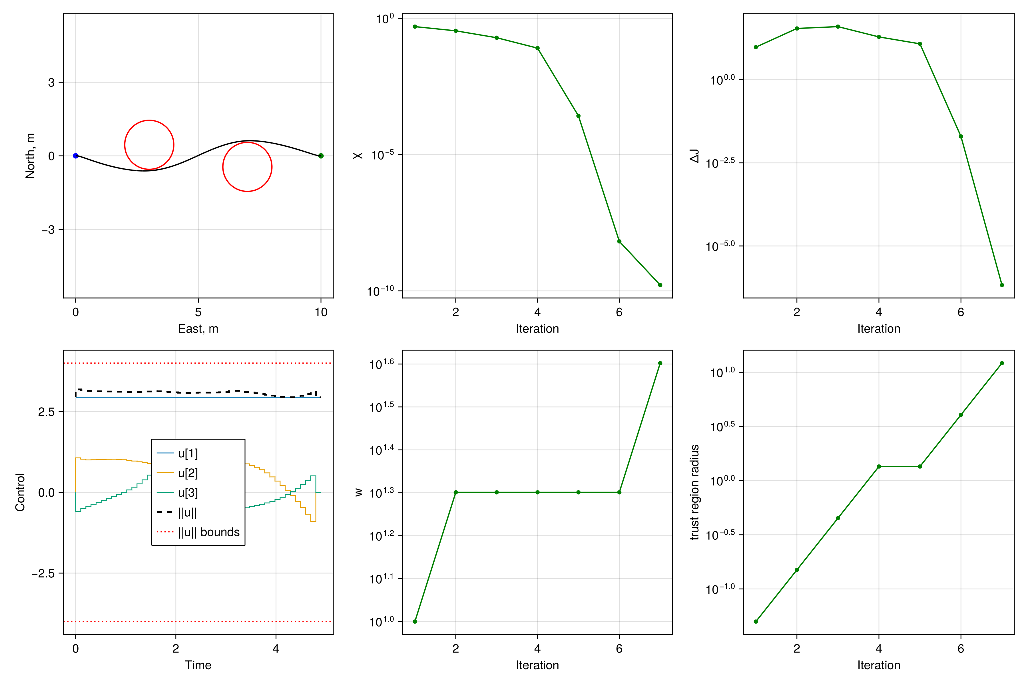
We can now visualize the solution
# propagate solution
sols_opt, g_dynamics_opt = SCPLib.get_trajectory(prob, solution.x, solution.u)

# get obstacles x[2] & x[3] values for plotting
coord_obstacle_1 = R_obstacle_1 * [cos.(LinRange(0, 2*pi, 100)) sin.(LinRange(0, 2*pi, 100))]' .+ p_obstacle_1[2:3]
coord_obstacle_2 = R_obstacle_2 * [cos.(LinRange(0, 2*pi, 100)) sin.(LinRange(0, 2*pi, 100))]' .+ p_obstacle_2[2:3]

# plot
fig = Figure(size=(1200,800))
ax2d = Axis(fig[1,1]; xlabel = "East, m", ylabel = "North, m", autolimitaspect=1)
scatter!(ax2d, [x_initial[2]], [x_initial[3]], color=:blue)
scatter!(ax2d, [x_final[2]], [x_final[3]], color=:green)
for (i, _sol) in enumerate(sols_opt)
    lines!(ax2d, Array(_sol)[2,:], Array(_sol)[3,:], color=:black)
end
lines!(ax2d, coord_obstacle_1[1,:], coord_obstacle_1[2,:], color=:red)
lines!(ax2d, coord_obstacle_2[1,:], coord_obstacle_2[2,:], color=:red)

# plot controls
ax_u = Axis(fig[2,1]; xlabel="Time", ylabel="Control")
for i in 1:3
    stairs!(ax_u, prob.times[1:end-1], solution.u[i,:], label="u[$i]", step=:pre, linewidth=1.0)
end
stairs!(ax_u, prob.times[1:end-1], solution.u[4,:], label="||u||", step=:pre, linewidth=2.0, color=:black, linestyle=:dash)
hlines!(ax_u, [-T_max, T_max], color=:red, linestyle=:dot, label="||u|| bounds")
axislegend(ax_u, position=:cc)

# plot iterate information
colors_accept = [solution.info[:accept][i] ? :green : :red for i in 1:length(solution.info[:accept])]
ax_χ = Axis(fig[1,2]; xlabel="Iteration", ylabel="χ", yscale=log10)
scatterlines!(ax_χ, 1:length(solution.info[:accept]), solution.info[:χ], color=colors_accept, marker=:circle, markersize=7)

ax_w = Axis(fig[2,2]; xlabel="Iteration", ylabel="w", yscale=log10)
scatterlines!(ax_w, 1:length(solution.info[:accept]), solution.info[:w], color=colors_accept, marker=:circle, markersize=7)

ax_J = Axis(fig[1,3]; xlabel="Iteration", ylabel="ΔJ", yscale=log10)
scatterlines!(ax_J, 1:length(solution.info[:accept]), abs.(solution.info[:ΔJ]), color=colors_accept, marker=:circle, markersize=7)

ax_Δ = Axis(fig[2,3]; xlabel="Iteration", ylabel="trust region radius", yscale=log10)
scatterlines!(ax_Δ, 1:length(solution.info[:accept]), [minimum(val) for val in solution.info[:Δ]], color=colors_accept, marker=:circle, markersize=7)

display(fig)