Basic Optimal Control Problem
We will start with a simple, fixed-time optimal control problem.
using Clarabel
using GLMakie
using JuMP
using LinearAlgebra
using OrdinaryDiffEq

using SCPLib
Define dynamics
We will first define and instantiate a struct that will hold the control, along with any parameters we may want to pass to the equations of motion:
# create parameters with `u` entry
mutable struct ControlParams
    μ::Float64
    u::Vector
    function ControlParams(μ::Float64)
        new(μ, zeros(4))
    end
end

μ = 1.215058560962404e-02
DU = 389703     # km
TU = 382981     # sec
MU = 500.0      # kg
VU = DU/TU      # km/s
params = ControlParams(μ)
We will now define an equations of motion
function eom!(drv, rv, p, t)
    x, y, z = rv[1:3]
    vx, vy, vz = rv[4:6]
    r1 = sqrt( (x+p.μ)^2 + y^2 + z^2 );
    r2 = sqrt( (x-1+p.μ)^2 + y^2 + z^2 );
    drv[1:3] = rv[4:6]
    # derivatives of velocities
    drv[4] =  2*vy + x - ((1-p.μ)/r1^3)*(p.μ+x) + (p.μ/r2^3)*(1-p.μ-x);
    drv[5] = -2*vx + y - ((1-p.μ)/r1^3)*y - (p.μ/r2^3)*y;
    drv[6] = -((1-p.μ)/r1^3)*z - (p.μ/r2^3)*z;
    # append controls
    drv[4:6] += p.u[1:3]
    return
end
Define problem
We will now define boundary conditions
rv0 = [1.0809931218390707E+00,
    0.0000000000000000E+00,
    -2.0235953267405354E-01,
    1.0157158264396639E-14,
    -1.9895001215078018E-01,
    7.2218178975912707E-15]
period_0 = 2.3538670417546639E+00

rvf = [1.1648780946517576,
    0.0,
    -1.1145303634437023E-1,
    0.0,
    -2.0191923237095796E-1,
    0.0]
period_f = 3.3031221822879884
We can now define the objective function
function objective(x, u)
    return sum(u[4,:])
end
We will now define the problem parameters
N = 100
nx = 6
nu = 4                              # [ux,uy,uz,Γ]
tf = 2.6
times = LinRange(0.0, tf, N)

thrust = 0.35    # N
umax = thrust/MU/1e3 / (VU/TU)
We will now define an initial guess by propagating the initial and final boundary conditions
# initial & final LPO
sol_lpo0 = solve(
    ODEProblem(eom!, rv0, [0.0, period_0], params),
    Tsit5(); reltol = 1e-12, abstol = 1e-12
)
sol_lpof = solve(
    ODEProblem(eom!, rvf, [0.0, period_f], params),
    Tsit5(); reltol = 1e-12, abstol = 1e-12
)

# create reference solution
x_along_lpo0 = sol_lpo0(LinRange(0.0, period_0, N))
x_along_lpof = sol_lpof(LinRange(0.0, period_f, N))
x_ref = zeros(nx,N)
alphas = LinRange(0,1,N)
for (i,alpha) in enumerate(alphas)
    x_ref[:,i] = (1-alpha)*x_along_lpo0[:,i] + alpha*x_along_lpof[:,i]
end
u_ref = zeros(nu, N-1)
then, we instantiate the problem struct
prob = SCPLib.ContinuousProblem(
    Clarabel.Optimizer,
    eom!,
    params,
    objective,
    times,
    x_ref,
    u_ref;
    ode_method = Vern7(),
)
set_silent(prob.model)              # we will silence the convex program
and we will append convex constraints to prob.model
# append boundary conditions
@constraint(prob.model, constraint_initial_rv, prob.model[:x][:,1] == rv0)
@constraint(prob.model, constraint_final_rv,   prob.model[:x][:,end] == rvf)

# append constraints on control magnitude
@constraint(prob.model, constraint_associate_control[k in 1:N-1],
    [prob.model[:u][4,k], prob.model[:u][1:3,k]...] in SecondOrderCone())
@constraint(prob.model, constraint_control_magnitude[k in 1:N-1],
    prob.model[:u][4,k] <= umax)
Instantiate algorithm & solve problem
We can now instantiate an algorithm and solve
algo = SCPLib.SCvxStar(nx, N; w0 = 1e4)
solution = SCPLib.solve!(algo, prob, x_ref, u_ref; maxiter = 100)
Solving OCP with SCvx* Algorithm (`・ω・´)
Feasibility tolerance tol_feas : 1.00e-06
Optimality tolerance tol_opt : 1.00e-04
Objective tolerance tol_J0 : -1.00e+16
Initial penalty weight w : 1.00e+04
Use L1 penalty : No
Iter | J0 | ΔJ_i | ΔL_i | χ_i | ρ_i | r_i | w | acpt. |
1 | -3.085e-10 | 5.319e+01 | 5.806e+01 | 1.043e-02 | 9.16e-01 | 5.00e-02 | 1.00e+04 | yes |
2 | 1.727e-11 | 1.980e+01 | 2.430e+01 | 5.612e-03 | 8.15e-01 | 1.50e-01 | 2.00e+04 | yes |
3 | 2.001e+00 | -6.762e+01 | 2.266e+01 | 2.469e-02 | -2.98e+00 | 4.50e-01 | 4.00e+04 | no |
4 | 2.001e+00 | -6.762e+01 | 2.266e+01 | 2.469e-02 | -2.98e+00 | 2.25e-01 | 4.00e+04 | no |
5 | 2.194e+00 | 1.125e+01 | 2.259e+01 | 8.513e-03 | 4.98e-01 | 1.13e-01 | 4.00e+04 | yes |
6 | 6.712e+00 | -2.341e+01 | 5.402e+01 | 1.198e-02 | -4.33e-01 | 1.13e-01 | 8.00e+04 | no |
7 | 6.682e+00 | 4.138e+01 | 5.393e+01 | 2.869e-03 | 7.67e-01 | 5.63e-02 | 8.00e+04 | yes |
8 | 8.502e+00 | -2.967e+02 | 2.179e+01 | 2.114e-02 | -1.36e+01 | 1.69e-01 | 1.60e+05 | no |
9 | 8.475e+00 | -3.237e+00 | 2.176e+01 | 3.462e-03 | -1.49e-01 | 8.44e-02 | 1.60e+05 | no |
10 | 8.476e+00 | 2.056e+01 | 2.168e+01 | 2.079e-03 | 9.48e-01 | 4.22e-02 | 1.60e+05 | yes |
11 | 8.263e+00 | -1.425e+01 | 5.732e+00 | 3.804e-03 | -2.49e+00 | 1.27e-01 | 3.20e+05 | no |
12 | 8.263e+00 | -1.425e+01 | 5.732e+00 | 3.804e-03 | -2.49e+00 | 6.33e-02 | 3.20e+05 | no |
13 | 8.268e+00 | 3.471e+00 | 5.719e+00 | 1.496e-03 | 6.07e-01 | 3.16e-02 | 3.20e+05 | yes |
14 | 8.235e+00 | 1.147e+01 | 1.148e+01 | 5.480e-04 | 9.99e-01 | 3.16e-02 | 6.40e+05 | yes |
15 | 8.211e+00 | 2.210e+00 | 2.211e+00 | 1.404e-05 | 9.99e-01 | 9.49e-02 | 1.28e+06 | yes |
16 | 8.211e+00 | -3.579e-02 | 2.356e-03 | 5.955e-05 | -1.52e+01 | 2.85e-01 | 2.56e+06 | no |
17 | 8.211e+00 | -3.580e-02 | 2.356e-03 | 5.956e-05 | -1.52e+01 | 1.42e-01 | 2.56e+06 | no |
18 | 8.211e+00 | -3.581e-02 | 2.356e-03 | 5.957e-05 | -1.52e+01 | 7.12e-02 | 2.56e+06 | no |
19 | 8.211e+00 | -3.581e-02 | 2.356e-03 | 5.956e-05 | -1.52e+01 | 3.56e-02 | 2.56e+06 | no |
Iter | J0 | ΔJ_i | ΔL_i | χ_i | ρ_i | r_i | w | acpt. |
20 | 8.211e+00 | -3.580e-02 | 2.356e-03 | 5.955e-05 | -1.52e+01 | 1.78e-02 | 2.56e+06 | no |
21 | 8.211e+00 | -3.578e-02 | 2.356e-03 | 5.954e-05 | -1.52e+01 | 8.90e-03 | 2.56e+06 | no |
22 | 8.211e+00 | -2.800e-03 | 2.259e-03 | 1.760e-05 | -1.24e+00 | 4.45e-03 | 2.56e+06 | no |
23 | 8.212e+00 | 1.682e-03 | 2.056e-03 | 1.853e-06 | 8.18e-01 | 2.22e-03 | 2.56e+06 | yes |
24 | 8.211e+00 | -5.020e-03 | 3.791e-04 | 1.506e-05 | -1.32e+01 | 6.67e-03 | 5.12e+06 | no |
25 | 8.211e+00 | -2.623e-03 | 3.759e-04 | 1.058e-05 | -6.98e+00 | 3.34e-03 | 5.12e+06 | no |
26 | 8.211e+00 | 1.677e-04 | 3.210e-04 | 1.108e-06 | 5.22e-01 | 1.67e-03 | 5.12e+06 | yes |
27 | 8.211e+00 | -7.971e-05 | 2.599e-04 | 1.616e-06 | -3.07e-01 | 1.67e-03 | 1.02e+07 | no |
28 | 8.211e+00 | 2.199e-04 | 2.325e-04 | 9.000e-07 | 9.46e-01 | 8.34e-04 | 1.02e+07 | yes |
29 | 8.211e+00 | -1.211e-03 | 7.310e-05 | 3.910e-06 | -1.66e+01 | 2.50e-03 | 2.05e+07 | no |
30 | 8.211e+00 | -1.498e-04 | 6.814e-05 | 1.409e-06 | -2.20e+00 | 1.25e-03 | 2.05e+07 | no |
31 | 8.211e+00 | 4.314e-05 | 5.283e-05 | 6.349e-08 | 8.17e-01 | 6.26e-04 | 2.05e+07 | yes |
Status : Optimal
Iterations : 31
Total CPU time : 2.08 sec
Objective : 8.2112e+00
Objective improvement ΔJ : 4.3138e-05 (tol: 1.0000e-04)
Max constraint violation : 6.3492e-08 (tol: 1.0000e-06)Analyze solution
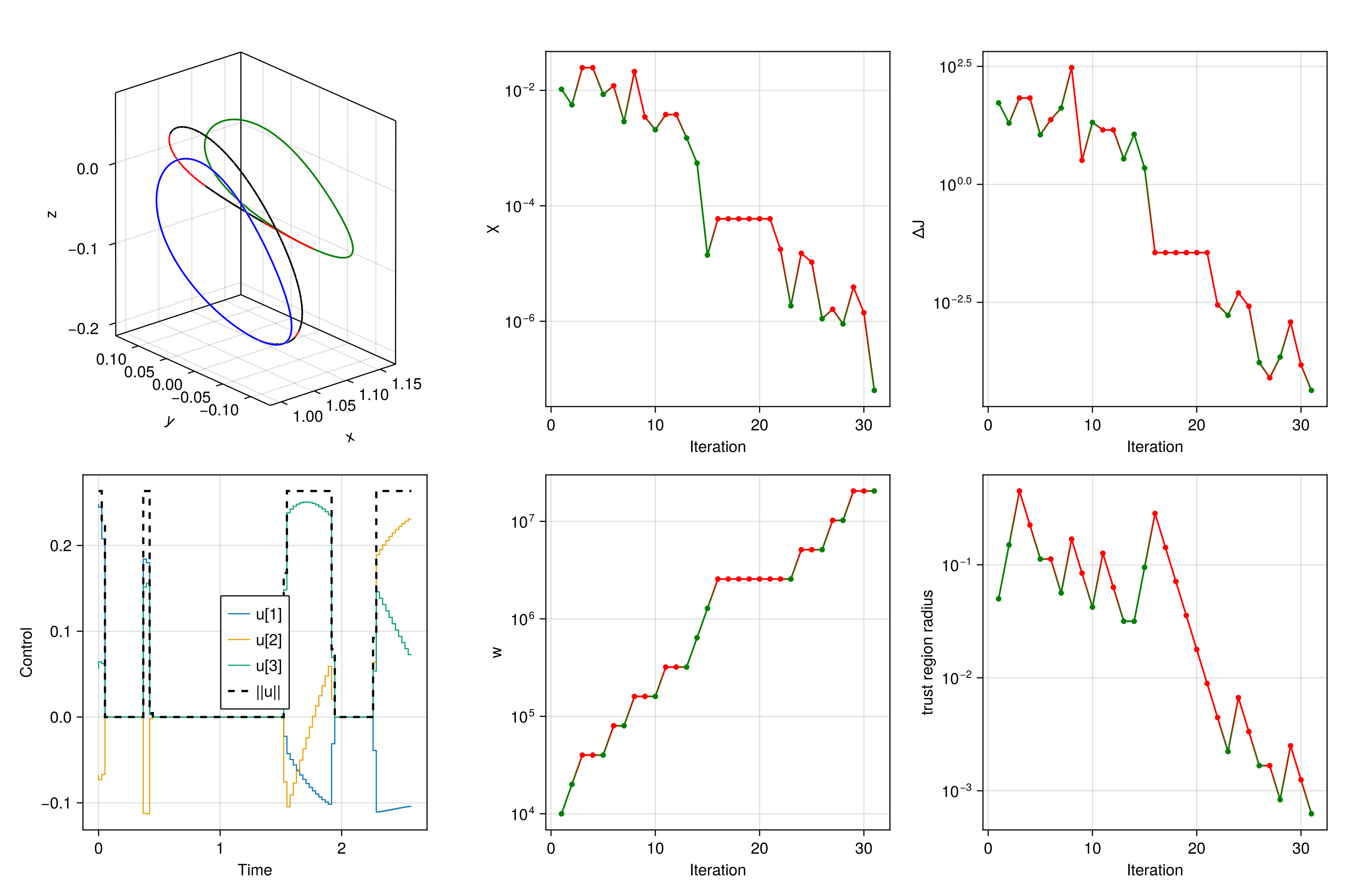
We can now visualize the solution
# propagate controlled trajectory solution
sols_opt, g_dynamics_opt = SCPLib.get_trajectory(prob, solution.x, solution.u)
arc_colors = [
    solution.u[4,i] > 1e-6 ? :red : :black for i in 1:N-1
]
for (i, _sol) in enumerate(sols_opt)
    lines!(ax3d, Array(_sol)[1,:], Array(_sol)[2,:], Array(_sol)[3,:], color=arc_colors[i])
end

# plot controls
ax_u = Axis(fig[2,1]; xlabel="Time", ylabel="Control")
for i in 1:3
    stairs!(ax_u, prob.times[1:end-1], solution.u[i,:], label="u[$i]", step=:pre, linewidth=1.0)
end
stairs!(ax_u, prob.times[1:end-1], solution.u[4,:], label="||u||", step=:pre, linewidth=2.0, color=:black, linestyle=:dash)
axislegend(ax_u, position=:cc)

# plot iterate information
colors_accept = [solution.info[:accept][i] ? :green : :red for i in 1:length(solution.info[:accept])]
ax_χ = Axis(fig[1,2]; xlabel="Iteration", ylabel="χ", yscale=log10)
scatterlines!(ax_χ, 1:length(solution.info[:accept]), solution.info[:χ], color=colors_accept, marker=:circle, markersize=7)

ax_w = Axis(fig[2,2]; xlabel="Iteration", ylabel="w", yscale=log10)
scatterlines!(ax_w, 1:length(solution.info[:accept]), solution.info[:w], color=colors_accept, marker=:circle, markersize=7)

ax_J = Axis(fig[1,3]; xlabel="Iteration", ylabel="ΔJ", yscale=log10)
scatterlines!(ax_J, 1:length(solution.info[:accept]), abs.(solution.info[:ΔJ]), color=colors_accept, marker=:circle, markersize=7)

ax_Δ = Axis(fig[2,3]; xlabel="Iteration", ylabel="trust region radius", yscale=log10)
scatterlines!(ax_Δ, 1:length(solution.info[:accept]), [minimum(val) for val in solution.info[:Δ]], color=colors_accept, marker=:circle, markersize=7)

display(fig)